The idea: the order of a product changes its cost
To compute a product of several matrices A1 × A2 × … × An you multiply two at a time. Matrix multiplication is associative: (A1A2)A3 and A1(A2A3) give the same matrix. But they do not cost the same. The matrix chain problem asks for the order, the parenthesization, that needs the fewest scalar multiplications. The page solves it with dynamic programming: a cost table filled from short chains to long ones, and a split table that remembers where each best order splits.
The cost of one product
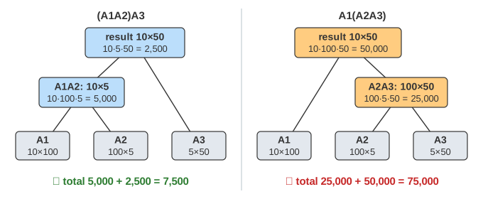
Write the sizes as a list of dimensions p0, p1, …, pn: matrix Ai is pi−1 × pi, so neighbours fit together. Multiplying a p × q matrix by a q × r matrix with the school method computes p·r entries, each a sum of q products: p·q·r multiplications, and the result is p × r. With 10×100, 100×5 and 5×50, doing A1A2 first leaves a small 10×5 matrix; doing A2A3 first builds a big 100×50 one. (Demo: 3 matrices, (AB)C vs A(BC))
Why not try every order?
Every order has a last multiplication, which splits the chain into a left part and a right part, each ordered in its own way. Counting the orders this way gives the Catalan numbers: n matrices have Cn−1 orders.
| matrices n | 3 | 4 | 6 | 10 | 20 |
|---|---|---|---|---|---|
| orders Cn−1 | 2 | 5 | 42 | 4,862 | 1,767,263,190 |
The count grows about like 4n, so trying them all is only possible for tiny chains.
The recurrence: try every last split
Let m[i][j] be the fewest multiplications for Ai..Aj. If the best order's last multiplication splits at k, it multiplies the result of Ai..Ak (a pi−1 × pk matrix) by the result of Ak+1..Aj (pk × pj). Both parts must themselves be done in their cheapest way, or the whole would not be cheapest. This is optimal substructure. We don't know k, so we try them all:
m[i][i] = 0, m[i][j] = min over i ≤ k < j of m[i][k] + m[k+1][j] + pi−1·pk·pj
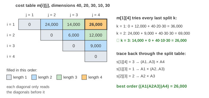
The split table s[i][j] stores the k that gave the minimum. On the canvas, the candidate list under the split table shows every k for the cell being filled; the blue and green cells are the two halves of the winning split, and the matrices in the chain are coloured the same way.
Filling by chain length
A cell m[i][j] reads only cells for shorter chains. So the page fills the table by length l = j − i + 1: first the diagonal (length 1, all zeros), then all chains of two matrices, then three, up to m[1][n], the answer. Each Step fills one cell. Filling row by row from the top would be wrong: m[1][3] needs m[2][3], which sits in a later row. (Demo: 4 matrices, fill the table by length)
Trace back: the split table gives the order
The cost table only says how cheap the best order is. To get the order itself, start at s[1][n] = k: the last multiplication is (A1..Ak) × (Ak+1..An). Then look up s for each half, and so on, until every part is a single matrix. The page shows unfinished parts in brackets, like ([A1..A3][A4..A6]). For the CLRS chain 30, 35, 15, 5, 10, 20, 25 the result is ((A1(A2A3))((A4A5)A6)) with 15,125 multiplications. (Demo: 6 matrices from CLRS)
The demos in numbers
| dimensions | best | best order | left to right | right to left | worst |
|---|---|---|---|---|---|
| 10, 100, 5, 50 | 7,500 | ((A1A2)A3) | 7,500 | 75,000 | 75,000 |
| 40, 20, 30, 10, 30 | 26,000 | ((A1(A2A3))A4) | 48,000 | 51,000 | 69,000 |
| 30, 35, 15, 5, 10, 20, 25 | 15,125 | ((A1(A2A3))((A4A5)A6)) | 40,500 | 47,500 | 58,000 |
| 100, 100, 100, 100, 1 | 30,000 | (A1(A2(A3A4))) | 2,010,000 | 30,000 | 2,010,000 |
| 5, 10, 3, 12, 5, 50, 6 | 2,010 | ((A1A2)((A3A4)(A5A6))) | 3,380 | 2,556 | 13,360 |
The fourth row is the everyday case of matrices times a vector, A·B·C·x: multiplying from the right keeps every intermediate result a vector, which is 67 times cheaper here. (Demo: matrices times a vector) The last row shows that the best order can be neither end first: it multiplies pairs in the middle and joins them. (Demo: the best order is balanced, neither end first) A greedy rule such as "always do the cheapest product first" can also miss the best order; only the table compares all splits.
Running time and space
There are n(n − 1)/2 cells above the diagonal, and a cell for a chain of length l tries l − 1 splits. In total that is (n³ − n)/6 split checks, Θ(n³) time, and Θ(n²) space for the two tables: 35 checks for 6 matrices instead of 42 whole orders, and 1,330 checks for 20 matrices instead of 1.7 billion orders. The same "interval DP" shape, a table over ranges filled by length with a split in the middle, also solves optimal binary search trees, polygon triangulation and parsing with CYK.
See also Matrix Multiplication for what one product computes, Longest Common Subsequence and 0/1 Knapsack for other dynamic-programming tables with a trace back.
What the page leaves out
Chains are capped at 6 matrices and dimensions at 200 so both tables fit on the canvas. The page counts only scalar multiplications of the school method; it leaves out additions, memory traffic and cache effects, faster multiplication algorithms such as Strassen's, the memoized top-down version of the same recurrence, and Hu and Shing's O(n log n) algorithm for this problem.