Mixture of Experts: Routing Tokens to Experts

The idea: many FFNs, but each token uses only a few

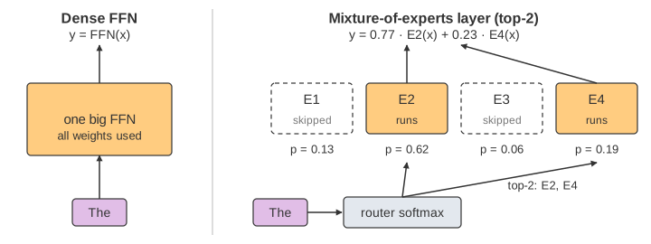
In a transformer block, the feed-forward network (FFN) after attention holds most of the weights. A mixture-of-experts (MoE) layer replaces that one FFN by several smaller FFNs called experts, plus a tiny router that decides, for every token, which experts run. Only the chosen experts do any work, so the model can store many more parameters without spending more compute per token.

The canvas follows 8 tokens, The cat sat on 3 + 4 =, through one MoE layer with 4 experts. Mixtral 8×7B, DeepSeek-V3 and (reportedly) GPT-4 are built this way. Where the layer sits inside a whole model is on How a Large Language Model Works; the attention layer that comes before it is on Self-Attention.

The router: a linear layer and a softmax

The router is a single weight matrix W_r with one column per expert. For a token vector x it computes the scores z = x · W_r and turns them into probabilities with softmax: p_i = e^z_i / Σ e^z. For cat the scores are [2.0, 0.3, −0.2, 1.0] and the probabilities [0.60, 0.11, 0.07, 0.22]. The router is trained with the rest of the model, so it learns which experts are good for which tokens. (Demo 1: one token through the router)

Top-k and the gate weights

Only the top-k experts by probability run. The layer's output is their weighted sum y = Σ g_i · E_i(x), added back to x by the residual connection.

• k = 2 (GShard, Mixtral): the two probabilities are renormalized to add up to 1. cat keeps E1 (0.60) and E4 (0.22), so g = 0.73 and 0.27.
• k = 1 (Switch Transformer): one expert, and the gate weight is the probability itself, g = p. Multiplying by p is what lets the gradient reach the router.

The experts that were not chosen are never computed for this token. That is the "sparse" in sparse MoE.

Capacity and overflow

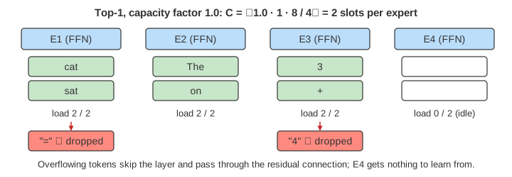
In a large model each expert lives on its own GPU, and the hardware wants fixed-size buffers. So every expert gets a fixed number of slots per batch, its expert capacity:

C = ⌈capacity_factor · k · N / E⌉

k · N / E is the fair share (here 2 · 8 / 4 = 4 assignments per expert); the capacity factor adds headroom. Assignments are dispatched in order: first every token's first choice, then every second choice. When an expert is full, the next assignment overflows: the token is dropped for that expert and skips it. A token that loses all its experts passes through on the residual connection alone, unchanged by the layer.

Setting	C	Loads E1–E4	Dropped
top-2, capacity factor 1.25	5	4 3 4 5	none
top-2, capacity factor 1.0	4	4 3 4 4	3 → E4
top-1, capacity factor 1.0	2	2 2 2 0	4 → E3, = → E1

A larger capacity factor drops fewer tokens but wastes memory and compute on empty slots; Switch Transformer used 1.0–1.25 in training. (Demo 2: a batch, top-2, capacity 1.25; Demo 3: top-1, capacity 1.0: overflow)

The load-balancing loss

Left alone, the router tends to collapse: a few experts get slightly better early on, get more tokens, get trained more and win even more often. The others sit idle, and the busy ones overflow. With the collapsed router on the canvas, E1 gets every token's first choice and drops +, 4 and =. (Demo 4: collapsed router, balancing loss)

Switch Transformer adds an auxiliary loss to the training loss:

L_aux = E · Σ_i f_i · P_i

Here f_i is the share of assignments that chose expert i and P_i is its mean router probability over the batch. When both are 1/E for every expert, L_aux = 1; it grows when the counts and the probabilities pile up on the same experts (the trained router scores 0.98). The collapsed router has f_1 = 0.50, P_1 = 0.69 and L_aux = 1.60. f is a count and has no gradient, but P does: ∂L/∂z_tj = (E/N) · p_tj · (f_j − Σ_i f_i p_ti), which pushes down the scores of experts with f above average. The real loss is multiplied by a small coefficient (α = 0.01); the canvas takes big steps so the effect shows in two: L_aux goes 1.60 → 1.37 → 1.03 and no token is dropped any more. (Demo 5: training with the aux loss)

Sparse vs dense compute

Join the 4 experts into one FFN with a 4× wider hidden layer and you get a dense layer with exactly the same parameters. It runs every weight for every token: 8 × 4 = 32 expert-sized passes for the batch. The top-2 MoE runs 16, half the work. With more experts the gap grows: total parameters scale with E, compute per token only with k. (Demo 6: sparse vs dense compute)

Model	Experts per layer	k	Total params	Active per token
This page	4	2	4 FFNs	2 FFNs
Switch Transformer	up to 2,048	1	1.6 T	about one FFN
Mixtral 8×7B	8	2	47 B	13 B
DeepSeek-V3	256 routed + 1 shared	8	671 B	37 B

The catch is memory: every expert must be loaded, so an MoE needs the memory of its total size while running at the speed of its active size. Moving tokens between GPUs (all-to-all communication) also costs time. See also LoRA and Quantization for shrinking that memory, and Softmax & Cross-Entropy for the softmax the router uses.

What the page leaves out

The token vectors and the experts' own math (each expert is an ordinary FFN, see Neural Network Forward Pass). Real experts do not specialize in neat topics like "numbers"; their split is learned and hard to read. Also left out: noisy top-k gating, the router z-loss, expert-choice routing (experts pick tokens, so nothing overflows), DeepSeek's shared expert and bias-based balancing without an auxiliary loss, dropless kernels such as MegaBlocks, expert parallelism across GPUs, and the gradient flowing into W_r rather than straight into the scores.

References

Fedus, Zoph, Shazeer (2021) — Switch Transformers

Shazeer et al. (2017) — Outrageously Large Neural Networks: The Sparsely-Gated Mixture-of-Experts Layer

Jiang et al. (2024) — Mixtral of Experts

Hugging Face — Mixture of Experts Explained