The idea: one neuron draws one line
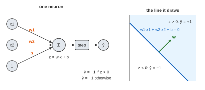
A perceptron (Rosenblatt, 1958) is a single artificial neuron. It takes inputs x1 and x2, multiplies each by a weight, adds a bias b, and passes the sum through a step activation: z = w1·x1 + w2·x2 + b, and the output is ŷ = +1 if z > 0, otherwise −1. The inputs where z = 0 form a straight line, the decision line. Points on one side get +1, points on the other side get −1. The weight vector w = (w1, w2) is perpendicular to the line and points to the + side; b shifts the line without turning it.
The learning rule
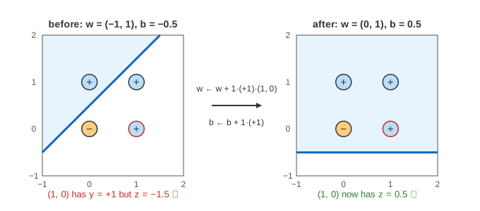
Training visits the points one at a time, in a fixed order. One pass over all points is an epoch. For a point x with label y (+1 or −1), the neuron is right when y and z have the same sign, so a mistake is y·z ≤ 0 (a point exactly on the line counts as a mistake). Correct points change nothing. A mistake changes the weights:
w ← w + η·y·x
b ← b + η·y
η is the learning rate. After the update, z for the same point grows by η·y·(‖x‖² + 1), in the direction of its label: the line rotates (w changes) and shifts (b changes) toward putting the point on its correct side. One update may not be enough, and it may push other points to the wrong side; the next epoch fixes those. Press Next Point to see the four parts: take the point, feed it in, compute z and ŷ, update.
Convergence on separable data
Data is linearly separable when some line has every + point on one side and every − point on the other. The perceptron convergence theorem says that then the rule makes a finite number of mistakes: at most (R/γ)², where R is the largest ‖x‖ and γ is the margin of the best separating line. After that, a whole epoch passes with no mistake and the weights never change again.
| data (η = 1, start w = (−1, 1), b = 0.5) | separable? | result | final line |
|---|---|---|---|
| AND (only (1, 1) is +) | yes | converged at epoch 7, 13 updates | 2·x1 + x2 − 2.5 = 0 |
| OR (only (0, 0) is −) | yes | converged at epoch 4, 5 updates | x1 + x2 − 0.5 = 0 |
| separable cloud (12 points) | yes | converged at epoch 3, 6 updates | 0.1·x1 + 2.2·x2 − 1.5 = 0 |
| XOR | no | cycles: epoch 4 starts where epoch 3 did | none |
The line it finds is just the first one that works, not the best one: it often passes close to a point. (Demo 1: AND, Demo 2: OR, Demo 3: separable cloud)
XOR: no line works
XOR is +1 when exactly one input is 1: (0, 1) and (1, 0) are +, (0, 0) and (1, 1) are −. The two + points sit on one diagonal and the two − points on the other, so any line that puts both + points on one side also takes at least one − point with it. The perceptron then keeps making mistakes. Because the weights only move in fixed steps, they come back to exactly the values they had at the start of an earlier epoch, and from there the same epoch repeats forever. The page detects this and stops. (Demo 4: XOR never converges) Minsky and Papert's 1969 book Perceptrons made this limit famous.
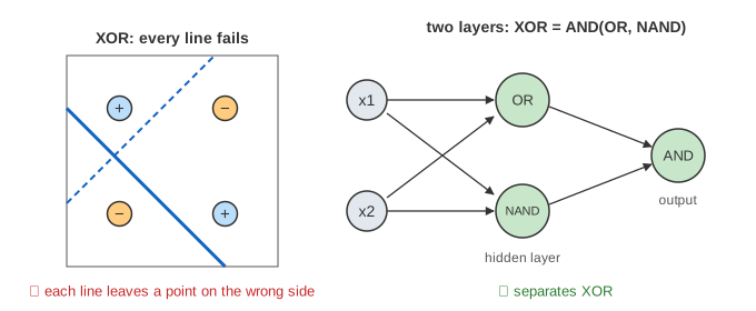
The fix is a hidden layer: h1 = OR(x1, x2) and h2 = NAND(x1, x2) are each separable, and XOR = AND(h1, h2). The step function has no useful derivative, so a multi-layer network uses a smooth activation (sigmoid, ReLU) and learns all layers with backpropagation: see Backpropagation, which trains a small network on exactly this XOR data.
The learning rate and the start
If training starts at w = 0, b = 0, η does not matter at all: every weight is a sum of η·y·x terms, so changing η only scales w and b, and the line, the mistakes and the epoch count stay the same. The page starts from w = (−1, 1), b = 0.5 instead, a line that is wrong for some points. Then η decides how far each update moves the line away from that start. On AND, η = 0.1 needs 20 epochs and η = 1 needs 7. (Demo 5: learning rate)
From perceptron to neural networks
| model | activation | learns by | output |
|---|---|---|---|
| perceptron | step | update on mistakes only | a class, ±1 |
| logistic regression | sigmoid | gradient of log loss, every point | a probability |
| multi-layer network | ReLU, sigmoid, … | backpropagation | any shape of boundary |
See also Linear and Logistic Regression, Neural Network Forward Pass, Gradient Descent and Backpropagation.
See also Train a Tiny Network on Your Points: add hidden neurons and their lines bend together into a boundary that can solve XOR.
See also Logistic Regression: the same line with a sigmoid, where every point pushes the weights by p − y instead of only mistakes.
The Support Vector Machine picks the best one instead: the line with the widest margin.
What the page leaves out
Only two inputs, so the boundary can be drawn; with n inputs it is a hyperplane. Real training shuffles the points each epoch; the page keeps a fixed order so every run is the same. Variants such as the averaged and the voted perceptron, the pocket algorithm for non-separable data, the kernel perceptron, and multi-class perceptrons are not shown.