The idea: one sample, one interval
We want the average height μ of all adults, but we can only measure a sample of n people. Their mean x̄ is our best guess, yet a different sample would give a different x̄. A confidence interval turns that one guess into a range, x̄ ± a margin, wide enough that the recipe catches the true μ in a chosen share of samples, the confidence level.
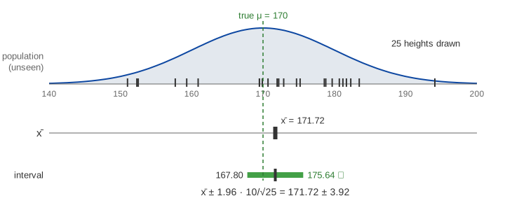
The page models heights as normal with μ = 170 cm and σ = 10 cm. The canvas knows μ so it can colour each interval, green if it contains μ and red if it misses; in real life μ is exactly what we don't know. The samples come from a seeded random generator, so every demo gives the same numbers each time.
The recipe
With σ known, the interval for a sample of n values is
x̄ ± z* · σ / √n SE = σ / √n, E = z* · SEThe standard error SE is how much x̄ wobbles from sample to sample, and the margin of error E is z* standard errors. For n = 25 and 95%: SE = 10/5 = 2 and E = 1.96 × 2 = 3.92, so every interval is 7.84 cm wide. Sample #1 has x̄ = 171.72, giving [167.80, 175.64] (Demo: one sample → one interval).
Why about 95% of the intervals catch μ
By the central limit theorem, x̄ over many samples is normal with mean μ and standard deviation SE. 95% of a normal lies within 1.96 standard deviations of its centre, so in 95% of samples x̄ lands within E of μ. And "x̄ is within E of μ" is the same statement as "μ is within E of x̄", which is exactly "the interval contains μ". On the canvas the light blue band is μ ± E: an interval turns red exactly when its x̄ dot falls outside the band.
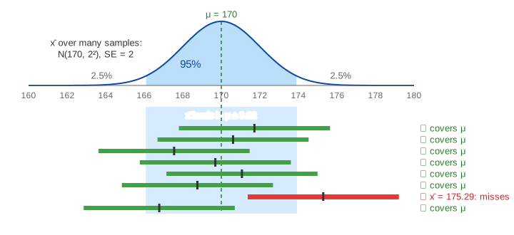
With seed 2475, 19 of the first 20 intervals contain μ; sample #11 (x̄ = 175.29, 5.29 cm above μ) misses (Demo: 20 intervals, one misses). After 100 samples, 95 contain μ and #11, #43, #49, #64 and #78 miss (Demo: 100 intervals → 95 cover μ). Over a short run the count wanders: 18 or 20 out of 20 is just as normal as 19.
Bigger n: narrower intervals
SE = σ/√n shrinks as the sample grows, so the interval narrows like 1/√n: four times the data halves the width. The coverage does not change, because the margin shrinks exactly as fast as the wobble of x̄ (Demo: bigger n → narrower: 19 of 20 cover at n = 5 and at n = 100, and the narrow n = 100 rows sit under the faded wide n = 5 rows).
| n | SE = 10/√n | 95% width 2E |
|---|---|---|
| 5 | 4.47 | 17.53 cm |
| 10 | 3.16 | 12.40 cm |
| 25 | 2.00 | 7.84 cm |
| 100 | 1.00 | 3.92 cm |
Higher confidence: wider intervals
z* is the number with the chosen share of the standard normal between −z* and z*. Asking to miss less often means a bigger z* and a wider interval (Demo: 80% vs 99% confidence: at 80%, 16 of 20 intervals contain μ; at 99%, all 20 do, but each is twice as wide).
| Level | z* | Misses | Width at n = 25 |
|---|---|---|---|
| 80% | 1.28 | 1 in 5 | 5.13 cm |
| 90% | 1.645 | 1 in 10 | 6.58 cm |
| 95% | 1.96 | 1 in 20 | 7.84 cm |
| 99% | 2.576 | 1 in 100 | 10.30 cm |
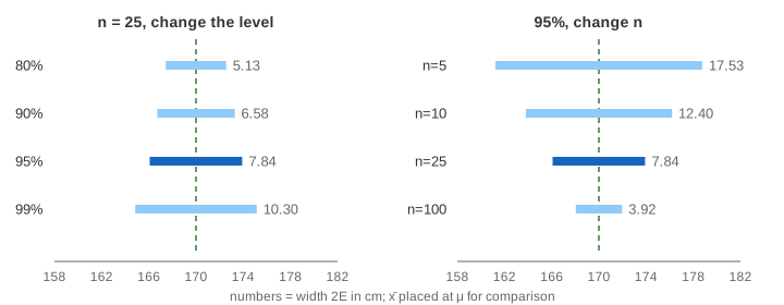
So precision and confidence pull against each other for a fixed n. The only way to get a narrow interval and a high level is a bigger sample: to halve the width at the same level, take four times as many people.
What "95% confidence" means
The 95% belongs to the method. Before the sample is drawn, the recipe has a 95% chance to produce an interval that contains μ. After it is drawn, μ is a fixed number and the interval is fixed too: it either contains μ or it does not. Saying "μ is in [167.80, 175.64] with probability 95%" mixes the two up; a probability for μ itself needs a prior, the Bayesian view (a credible interval).
The same intervals decide A/B tests: if the 95% interval for the difference between two variants excludes 0, the difference is significant at the 5% level. See also Normal Distribution, z-Scores and Confidence Intervals for the z table behind z*, and Monte Carlo estimation of π, where the error of an estimate also shrinks like 1/√n.
What the page leaves out
- Unknown σ: with the sample standard deviation s in place of σ, z* is replaced by Student's t with n − 1 degrees of freedom (2.78 for n = 5, 2.06 for n = 25), so small samples get wider intervals.
- Intervals for proportions (p̂ ± z*·√(p̂(1 − p̂)/n)), differences of means and regression slopes.
- Skewed or heavy-tailed data at small n, and the bootstrap, which builds intervals by resampling.
- One-sided intervals and the link to hypothesis tests and p-values.
- Bayesian credible intervals, which do give a probability for μ.