The idea: a small window of weights slides over the image
A convolutional layer does not connect every pixel to every neuron. It uses one small grid of weights, the kernel (or filter), here 3×3. The kernel is placed on the top-left corner of the image, the 9 pixels under it are multiplied by the 9 weights, and the 9 products are added up. That one number is one cell of the output, the feature map. Then the kernel moves one step and does the same again, until it has visited every position.
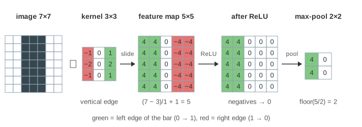
The page shows one channel and one kernel. The input is a 7×7 image of 0s and 1s (dark cells are 1). Press Next Position to see one position in detail, Finish Map for the rest, then ReLU and Max Pool. The selects pick the image, the kernel, the padding and the stride; changing one starts a new map.
One position: multiply element-wise, then add
For output cell (i, j) with stride s, the kernel's top-left corner sits on input pixel (i·s, j·s):
out[i][j] = Σ_a Σ_b x[i·s + a][j·s + b] · w[a][b] (a, b = 0, 1, 2)
The orange frame on the input marks the 9 pixels, the pixel × weight grid shows the 9 products, and the Σ box flies to its cell. On the vertical bar with the vertical-edge kernel, position (0, 0) covers columns 0–2. Only column 2 is ink, and its weights are 1, 2, 1, so the sum is 4 (Demo 1: edge detection, one position at a time).
A real layer also adds a bias to every cell. The page leaves it at 0.
Kernels are feature detectors
The weights decide what the layer responds to. A cell is large when the pixels under the kernel look like the kernel: positive weights on bright pixels, negative weights on dark ones.
| kernel | weights | responds to |
|---|---|---|
| vertical edge (Sobel x) | -1 0 1 / -2 0 2 / -1 0 1 | brighter to the right (+) or to the left (−) |
| horizontal edge (Sobel y) | -1 -2 -1 / 0 0 0 / 1 2 1 | brighter downwards (+) or upwards (−) |
| blur (Gaussian) | 1 2 1 / 2 4 2 / 1 2 1, ÷ 16 | nothing in particular: a weighted average, so edges get soft |
| sharpen | 0 -1 0 / -1 5 -1 / 0 -1 0 | differences from the neighbours, made stronger |
The two edge kernels add up to 0, so a flat area (all 0 or all 1) gives 0. Only a change gives a value. On the digit 7 the horizontal-edge kernel finds the top bar of the 7 and mostly ignores the vertical parts of the stroke (Demo 2: horizontal edges of the digit 7). Sharpen overshoots next to the stroke, above 1 on it and below 0 beside it (Demo 6: sharpen the digit 7).
In a CNN nobody writes these weights. They start random and are learned by gradient descent with backpropagation. The first layer of a trained image network usually ends up with edge- and colour-blob detectors much like these. See Backpropagation and Gradient Descent.
Stride, padding and the output size
The stride s is how far the kernel moves each time. With stride 2 it skips every other position, so the map is about half as wide (Demo 3: stride 2 shrinks the output).
Without padding the kernel cannot be centred on a border pixel, so a 3×3 kernel loses one pixel on each side: 7×7 becomes 5×5. This is "valid" padding. Zero padding adds p rings of zeros around the image first. With p = 1 the kernel can sit on every pixel and the output stays 7×7: "same" padding (Demo 4: zero padding keeps the size (same)). The border cells come out weaker (3 instead of 4 in the corners of the bar) because part of the window covers zeros.
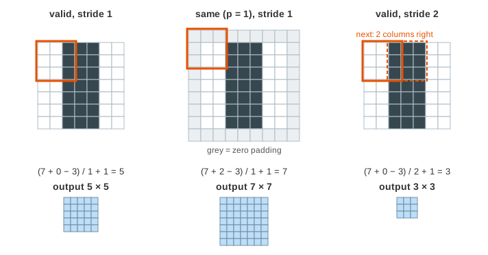
For an n×n input, a k×k kernel, padding p and stride s:
output size = floor((n + 2p − k) / s) + 1
| setting | formula | output |
|---|---|---|
| valid, stride 1 | (7 + 0 − 3) / 1 + 1 | 5 × 5 |
| same (p = 1), stride 1 | (7 + 2 − 3) / 1 + 1 | 7 × 7 |
| valid, stride 2 | (7 + 0 − 3) / 2 + 1 | 3 × 3 |
| same (p = 1), stride 2 | (7 + 2 − 3) / 2 + 1 | 4 × 4 |
"Same" means p = (k − 1) / 2 for an odd kernel: 1 for 3×3, 2 for 5×5. The canvas shows the formula with the current numbers under the panels.
ReLU
After the convolution comes an activation function, almost always ReLU: max(0, v). Negative cells become 0, positive cells stay. On the bar, the vertical-edge kernel says +4 on the left side and −4 on the right side; after ReLU only the left side is left (Demo 5: ReLU, then 2×2 max-pooling). A real layer has many kernels, so another kernel with the opposite signs would find the right side.
Without a non-linearity between them, two convolution layers in a row are just one bigger linear filter. ReLU is what lets stacked layers build more complex features. See Neural Network: the Forward Pass for activations in a plain network.
Max-pooling
Max-pooling with a 2×2 window and stride 2 cuts the map into 2×2 blocks and keeps the largest value of each. The map gets 4 times smaller, later layers see a larger part of the image per cell, and a feature that moves by one pixel often gives the same pooled value. Pooling has no weights to learn.
Its output size uses the same formula with k = 2, s = 2, p = 0: floor((m − 2) / 2) + 1 = floor(m / 2). A 5×5 map gives 2×2, and the last row and column, which fit no full block, are dropped. Average pooling takes the mean instead; many newer networks use a stride-2 convolution in place of pooling.
From one kernel to a CNN
A real convolutional layer repeats this for many kernels at once (32, 64, …), each giving its own feature map; together they are the output channels. A colour image has 3 input channels (R, G, B), so each kernel is 3×3×3 and sums over all channels. The weights are shared: the same 9 (or 27) numbers are used at every position, which is why a convolution has so few parameters compared with a fully connected layer, and why it finds a feature wherever it is in the image.
Strictly, what CNN libraries compute is cross-correlation: in mathematical convolution the kernel is flipped first. Since the weights are learned, the flip makes no difference, and the name stuck.
See also Neural Network: the Forward Pass, Backpropagation for how the kernel weights are learned, and Self-Attention for the other way modern networks mix information between positions.
Large convolutions are computed with the FFT: transform the image and the kernel, multiply bin by bin, transform back (see Fourier Series and the FFT).
See also CNN vs Transformer: how stacked 3×3 layers grow the receptive field, compared with self-attention reaching every patch in one layer.
What the page leaves out
Several input and output channels; the bias; learning the weights; average pooling and global pooling; dilated, depthwise and 1×1 convolutions; batch normalisation; grey-level images (the input is only 0s and 1s); and the stack of layers that ends in a fully connected classifier.