Draw a Digit Visualization | Neural Network Math & Backpropagation

The idea: your drawing in, ten numbers out, and every step is arithmetic

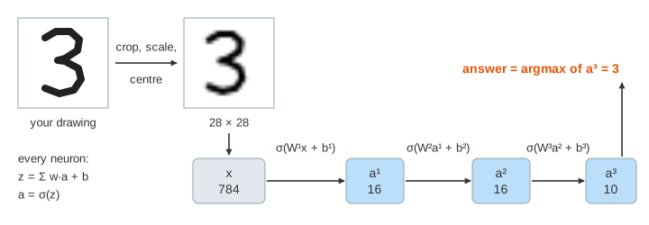
Draw a digit on the pad and press Recognize. The page turns the drawing into 784 numbers and runs them through a neural network with two hidden layers of 16 neurons and 10 output neurons, one per digit. This is the network from 3Blue1Brown's deep-learning lessons. Nothing is hidden. The right panel lists every weighted sum, bias and sigmoid the network computes. If the answer is wrong, pick the true digit and press Backprop Step. The page then works out the cost, runs backpropagation and takes one step of gradient descent, with all the numbers. Everything runs in your browser, in plain JavaScript. No server is involved.

A hand-drawn 3 on a pad is cropped, scaled and centred into a 28 by 28 image, read as 784 numbers x, then passes through hidden layer 1 (16 neurons), hidden layer 2 (16 neurons) and the output layer (10 neurons); the largest output, 3, is the answer — Pad → 28 × 28 → 784 numbers → 16 → 16 → 10 → the largest output is the answer. Each arrow between layers is a = σ(W·a + b).

From a drawing to 784 numbers

The network was trained on MNIST: 70,000 digits written by people, each a 28 × 28 grey image. In MNIST the digit was scaled to fit a 20 × 20 box and moved so that its centre of mass sits in the middle. Your drawing has to look the same, so the page repeats those steps (Demo: draw a 3, run every layer, step 0):

Crop to the ink: the smallest box (w × h pad pixels) around everything drawn.
Scale by s = 20 / max(w, h), so the longer side becomes 20 pixels, and put the box in the middle of 28 × 28. Each of the 784 pixels gets the average ink of the area it covers.
Centre: c_x = Σ x_i·col_i / Σ x_i and c_y = Σ x_i·row_i / Σ x_i. Then shift the image by round(13.5 − c_x), round(13.5 − c_y) pixels.
Read the 784 pixels row by row, i = 28·row + col: x_i = 0 for blank, 1 for full ink.

The input to the network is the vector x = (x₀, …, x₇₈₃). The network never sees strokes or shapes, only these 784 numbers. A digit drawn in a corner, or very small, would give a completely different vector. That is why the centring matters.

One neuron: weighted sum, bias, sigmoid

Every neuron in the hidden and output layers does the same two things with the activations a₁ … a_n of the layer before it. It has one weight w_i per input and one bias b:

z = w1·a1 + w2·a2 + … + wn·an + b        (the weighted sum plus the bias)
a = σ(z) = 1 / (1 + e^(−z))              (the sigmoid squeezes z into 0 … 1)

A positive weight means "I want this input on", a negative one "I want it off". The bias decides how big the sum must be before the neuron lights up: z > 0 gives a > 0.5. The sigmoid maps σ(−4) ≈ 0.02, σ(0) = 0.5 and σ(4) ≈ 0.98. For a first-layer neuron the 784 weights form a 28 × 28 picture. Neuron Math shows the picture, then the 784 products w_i·x_i. Blank pixels give 0, so only your ink counts. Then it shows the sum, the bias and σ (Demo: a hidden-1 neuron, 784 weights; Demo: output neuron "3" in full).

A small worked example with two inputs: w = (0.8, −0.5), a = (1, 0.6), b = −0.1 gives z = 0.8·1 + (−0.5)·0.6 − 0.1 = 0.4 and a = 1 / (1 + e^−0.4) = 0.599.

A layer is a matrix product

Writing the 16 neurons of a layer one under the other turns the 16 weighted sums into one matrix product. Row j of W holds neuron j's weights:

a¹ = σ(W¹·x  + b¹)     W¹: 16 × 784,  b¹: 16
a² = σ(W²·a¹ + b²)     W²: 16 × 16,   b²: 16
a³ = σ(W³·a² + b³)     W³: 10 × 16,   b³: 10

σ is applied to each entry separately. The whole network is one function of 784 numbers, a³ = σ(W³·σ(W²·σ(W¹·x + b¹) + b²) + b³), with this many numbers to choose:

Layer	Weights	Biases	Total
hidden 1	16 × 784 = 12,544	16	12,560
hidden 2	16 × 16 = 256	16	272
output	10 × 16 = 160	10	170
network	12,960	42	13,002

During the forward pass, the table in the right panel has one row per neuron j: Σ W·a (the weighted sum without the bias), + b, = z and a = σ(z).

Reading the answer

The answer is the output with the largest activation: argmax_k a³_k. The ten outputs are separate sigmoids, so they are not probabilities and need not add up to 1. A very unsure network may have every output below 0.5. Networks that need probabilities replace the last sigmoid with a softmax (see Neural Network Forward Pass). Softmax & Cross-Entropy shows that output layer in full: probabilities that add up to 1, and a gradient p − y with no σ' factor, so confident wrong answers are corrected fastest.

How wrong: the cost

To learn, the network needs a number that says how bad an answer is. For one example with true digit t, the wanted output is y = (0, …, 0, 1, 0, …, 0) with y_t = 1. The cost of this example is the sum of squared differences:

C = Σk (a³k − yk)²        k = 0 … 9

C is 0 only when output t is exactly 1 and every other output is 0. The cost of the whole network is the average of C over all training examples. Learning means finding the 13,002 weights and biases that make that average small.

Backpropagation: the chain rule, layer by layer

Gradient descent needs ∂C/∂w for every weight and ∂C/∂b for every bias: how fast C changes when that one number changes. For a weight w³_kj into output k, the change travels along a chain: w → z³_k → a³_k → C. So its derivative is a product of three local derivatives:

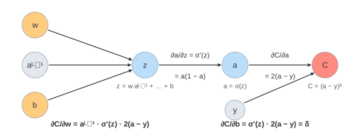
Each arrow has a simple local derivative. Multiply them along the path to get ∂C/∂w = a^(L−1) · σ'(z) · 2(a − y).

∂C/∂w3kj = ∂z3k/∂w3kj · ∂a3k/∂z3k · ∂C/∂a3k = a2j · σ'(z3k) · 2(a3k − yk)
σ'(z) = σ(z)·(1 − σ(z)) = a·(1 − a)

The product σ'(z)·∂C/∂a shows up again and again, so it gets a name: the neuron's error δ = ∂C/∂z. With it, all of backpropagation is four lines (⊙ means multiply entry by entry):

δ³ = 2(a³ − y) ⊙ a³(1 − a³)                       output layer
δˡ = ((Wˡ⁺¹)ᵀ · δˡ⁺¹) ⊙ aˡ(1 − aˡ)                 l = 2, then 1: going backwards
∂C/∂bˡj  = δˡj
∂C/∂Wˡji = δˡj · aˡ⁻¹i                              (a⁰ = x, the pixels)

The second line is the "back" in backpropagation. A neuron of hidden layer 2 affects C through all ten outputs, so its ∂C/∂a²_j is the sum Σ_k W³_kj·δ³_k. In 3Blue1Brown's words, the wishes of all the outputs are added up. The Backprop Step table shows exactly these columns: Σ W·δ, a(1 − a) and δ (Demo: cost and backprop on a 2).

The formulas match the lesson's three ways to raise an output's activation:

Lever	Derivative	What it says
its bias	∂C/∂b = δ	the simplest nudge, the same size as the error
its weights	∂C/∂w_i = δ·a_i	weights from bright neurons change most; blank inputs (a = 0) don't change at all ("neurons that fire together wire together")
the activations before it	∂C/∂a_i = Σ w_i·δ	push up inputs with positive weights, down those with negative weights. They can't be set directly, so this is passed back one layer.

The worked example continued, with true value y = 1: a = 0.599, so C = (0.599 − 1)² = 0.161, ∂C/∂a = 2(0.599 − 1) = −0.803, σ'(z) = 0.599 · 0.401 = 0.240, and δ = −0.193. Then ∂C/∂w₁ = δ·1 = −0.193, ∂C/∂w₂ = δ·0.6 = −0.116 and ∂C/∂b = −0.193.

One gradient step, and why mini-batches

The 13,002 partial derivatives together are the gradient ∇C. It points in the direction in which C grows fastest, so a small step the other way lowers C:

w ← w − η · ∂C/∂w        b ← b − η · ∂C/∂b        (learning rate η = 1 on this page)

In the example, w becomes (0.993, −0.384) and b becomes 0.093. Then z = 0.855, a = 0.702, and the cost falls from 0.161 to 0.089. On the page, Backprop Step does the same to all 13,002 numbers and runs your drawing again. The table compares a³ before and after (Demo: a 9 read as 1, one learning step: one step takes C from 1.84 to 0.73 and the answer from 1 to 9).

Learning from one example is not how a network is trained. Push hard enough on one drawing and the network starts reading other digits as that one. On this network, three steps with η = 3 on the 9 make it read the sample 2 and 3 as 9 too. Real training averages the gradient over many examples. Computing it over all 60,000 every step is slow, so stochastic gradient descent shuffles the data and averages over a mini-batch of a few dozen, then steps. Each step is a rougher estimate, but steps are far cheaper. See Gradient Descent, and Backpropagation Intuition for this network trained from random weights with mini-batches.

How these weights were trained

The weights were trained once, offline, by a plain JavaScript (Node.js) program. It ran the same forward pass and backpropagation as this page, with the same cost C = Σ (a − y)². The data was the 60,000 MNIST training images, each randomly shifted, rotated and scaled a little so that hand drawings work better. Mini-batches had 32 images. Instead of the plain step above, the training used Adam, a variant of gradient descent that adapts the step size for each parameter. After 30 passes over the data, the network reads 94.95 % of the 10,000 MNIST test digits correctly. That is about what 16-neuron sigmoid layers can do; larger networks reach 98 %, and convolutional networks 99.7 %. To keep the file small, the 12,544 first-layer weights are stored as 8-bit integers. The other numbers are rounded to 0.01. The page computes with exactly these stored numbers.

For the simplest classifier before neural networks, comparing your drawing with the average image of each digit (82 % on MNIST against this network's 94.95 %), see Draw a Digit: Template Matching.

To watch a network learn from scratch, small enough to see every weight as a line on a plot, see Train a Tiny Network on Your Points.

What the page leaves out

Training on the whole data set is not animated: the page takes one gradient step on one example, and the change is lost on Reset. Hidden neurons are not "edge" or "loop" detectors; what this kind of network really learns is shown on Neural Network: Recognizing Digits. Modern digit readers use ReLU, softmax with cross-entropy cost and convolutional layers (Convolution in a CNN); this page keeps the lesson's sigmoid and squared error. Your drawing is thicker or thinner than MNIST's pen strokes, and an unusual style (a 7 with a bar, a 4 with an open top) can still be misread. For the chain rule on a network small enough to follow every weight, see Backpropagation.