The idea: the model gives probabilities, the decoder picks the words
A language model does not write text. For a given beginning it only gives a probability for every possible next token. A decoding strategy turns those probabilities into text, one token at a time. The page runs three strategies on the same tiny model and the same prompt, in lockstep: each Step adds one token in every lane. Greedy takes the most likely token. Beam search keeps the 3 likeliest partial sentences. Top-p sampling draws a token at random from the likeliest few.
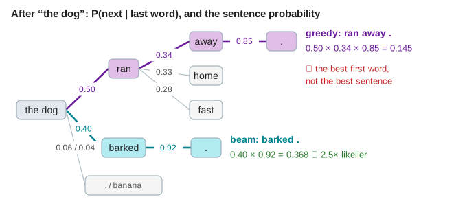
The model here is a bigram table: the probability of the next word depends only on the last word. It has 20 words and the end token “.”. Every row adds up to 1, and every row has a small tail, the junk word “banana”, which only careless sampling picks. A real model computes such a row with a transformer and a softmax over 50,000 or more tokens, but the decoders work the same way. The probability of a whole text is the product of its token probabilities: P(“the dog barked .”) = 0.40 × 0.92 = 0.368 after the prompt.
Greedy: the most likely token, every time
Greedy decoding takes the token with the highest probability, appends it and repeats. It needs one model call per token and always writes the same text for the same prompt. It is short-sighted: after “the dog” it takes “ran” (0.50) over “barked” (0.40), and then the best it can do is “away .” for a total of 0.145. (Demo: the dog)
It can also fall into a repetition loop. After “the cat” the most likely words are “sat”, “on”, “the”, “cat”, and then the same four again. Greedy writes “the cat sat on the cat sat on the cat” until the 8-token limit. Real models do this too, which is why plain greedy decoding is rarely used for open-ended text. (Demo: the cat — greedy loops)
Beam search: keep the k likeliest sentences
Beam search keeps the k best partial sentences, the beams (k = 3 here). Each step it extends every beam with every next token, scores each candidate by its sentence probability and keeps the k best. A beam that ends with “.” is finished and is carried over unchanged. Probabilities only shrink as a sentence grows, so when the best beam is finished nothing can beat it, and the search stops.
After “the cat” the beams after 2 steps are “sat on” 0.275, “sat down” 0.150 and “slept .” 0.128. Two steps later the looping beam “sat on the cat” has fallen to 0.088, and the finished “slept .” is the best: beam search escapes greedy's loop. The price is up to k model calls per token: 7 calls here against greedy's 8 for a much shorter text, and 7 against 3 for “a bird flew away .”, where all three lanes agree. (Demo: a bird — a sure model)
Beam search maximizes probability, and short texts are more probable. That is why it likes “slept .” and why real systems divide the log-probability by a power of the length (length normalization). It is the usual choice when there is one right answer, such as translation or speech recognition, and it is close to the Viterbi algorithm, which finds the single most likely path exactly when the model is a hidden Markov model.
Top-p sampling and temperature
Sampling draws the next token at random with its probability, so the text varies from run to run and can escape loops. Top-p, or nucleus sampling, first sorts the tokens and keeps the smallest set whose probabilities add up to p (0.9 here), then renormalizes them and draws. The cut adapts to the model: after “bird” it keeps only “flew” and “sat”, after “ran” it keeps three nearly equal words. The draws come from a seeded generator, so a seed always gives the same text and undo works.
Temperature T reshapes the probabilities first: each probability is raised to the power 1/T and the row is renormalized, which is the same as dividing the logits by T before the softmax. T < 1 makes the top token stronger: at T = 0.3, sampling after “the cat” writes greedy's loop. T > 1 flattens the row and the tail grows. (Demo: temperature 0.3)
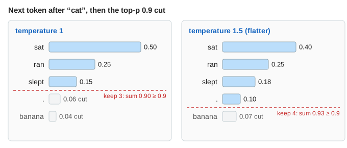
With T = 1.5 and no cut (top-p = 1), seed 37 writes “the cat ran banana banana .”. With the same seed and top-p 0.9 the random numbers are the same, but “banana” is no longer in the set, and it writes “the cat ran fast .”. (Demo: temperature 1.5, top-p off; Demo: temperature 1.5, top-p 0.9)
The demos in numbers
| demo | greedy | beam, k = 3 | top-p sampling |
|---|---|---|---|
| the cat | ✗ sat on the cat sat on the cat, 0.0077, 8 calls | ✓ slept ., 0.128, 7 calls | seed 11: sat on the dog barked ., 0.024 |
| the dog | ran away ., 0.145, 3 calls | ✓ barked ., 0.368, 3 calls | seed 8: ran home ., 0.149 |
| a bird | ✓ flew away ., 0.578, 3 calls | flew away ., 0.578, 7 calls | seed 1: flew away ., 0.578, 3 calls |
| T = 0.3 | (the cat loop) | (slept .) | seed 2: the same loop as greedy, 0.0077 |
| T = 1.5, top-p off | (the cat loop) | (slept .) | ✗ seed 37: ran banana banana ., 0.0015 |
| T = 1.5, top-p 0.9 | (the cat loop) | (slept .) | ✓ seed 37: ran fast ., 0.056 |
The numbers are P(text) after the prompt under the model (at T = 1), whatever strategy wrote the text.
When to pick which
| greedy | beam search | top-p sampling | |
|---|---|---|---|
| output | one fixed text | one fixed text, usually likelier | a different text per seed |
| cost | 1 model call per token | up to k calls per token, k beams in memory | 1 call per token |
| goes wrong | repetition loops, misses a better second choice | short, bland and repetitive text in open-ended writing | junk tokens when T is high and nothing is cut |
| use it for | short answers, code, tests that need the same output | translation, speech recognition, summaries | chat, stories, brainstorming |
See also How a Large Language Model Works, where a tiny GPT computes the next-token probabilities that these strategies decode, and Softmax & Cross-Entropy for how temperature reshapes a softmax.
See Speculative Decoding, where a small draft model guesses k tokens and the big model checks them in one pass without changing the output.
What the page leaves out
The model is a fixed bigram table, so the next word depends only on the last word; a real model looks at the whole context. The page leaves out top-k sampling, min-p and typical sampling, repetition and frequency penalties, length normalization and the end-of-sentence handling of real beam search libraries, diverse beam search, contrastive search, speculative decoding (a small model drafts, the big one checks) and the batching and KV cache that make each model call cheap.