The idea: guess what you cannot see from what you can
A friend in another city tells you what they did each day: walk, shop or clean. You never hear the weather, but you know they walk on sunny days and clean on rainy ones. Which weather sequence best explains what they did? That is decoding a hidden Markov model (HMM), and the Viterbi algorithm finds the single most likely hidden sequence without trying them all.
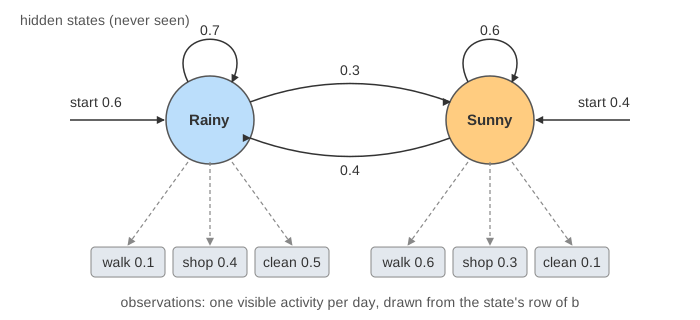
The model: π, a and b
- Hidden states: Rainy, Sunny. They form a Markov chain: tomorrow depends only on today.
- Start probabilities π: Rainy 0.6, Sunny 0.4.
- Transition probabilities a(i→j): the top-left table on the canvas. Weather tends to stay (0.7, 0.6).
- Emission probabilities b(state, observation): the second table. Each row sums to 1.
The probability of one hidden path together with the observations is a product: start, then one transition and one emission per day. For Sunny, Rainy, Rainy with walk, shop, clean: 0.4·0.6 × 0.4·0.4 × 0.7·0.5 = 0.01344.
The trellis and the recurrence
The trellis has one row per hidden state and one column per day. Cell δt(s) holds the probability of the best path that ends in state s on day t and produces the first t observations:
Day 1 is just π(s)·b(s, o1). For every later cell, two candidates arrive from the previous column (yellow boxes on the canvas); the bigger one wins and the cell remembers where it came from: the back-pointer (blue arrow). The loser is dropped for good: any best path through this cell must use the best way into it. (Demo: 3 days, step by step)
for s in states:            delta[1][s] = pi[s] * b[s][o1]
for t in 2..T:
    for s in states:
        i* = argmax_i delta[t-1][i] * a[i][s]
        delta[t][s] = delta[t-1][i*] * a[i*][s] * b[s][o_t]
        back[t][s]  = i*
s = argmax_s delta[T][s]                  # traceback
for t in T..2:  path[t] = s;  s = back[t][s]
path[1] = s
Traceback
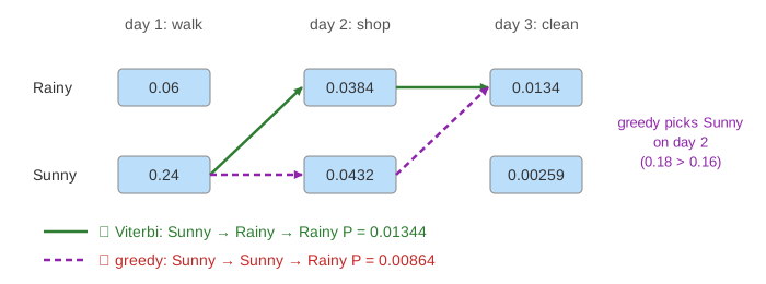
When the last column is full, the best path ends in its bigger cell. Follow the back-pointers right to left and you read the whole path (green). For walk, shop, clean that is Sunny → Rainy → Rainy with P = 0.01344. Notice day 2: the Sunny cell (0.0432) is bigger than the Rainy cell (0.0384), yet the best path goes through Rainy, because only Rainy leads well into "clean" on day 3. The path comes from the back-pointers, not from the biggest cell in each column.
Why it is dynamic programming
With N states and T days there are NT hidden paths: 28 = 256 for the 8-day sequence, and 10100 for 100 days with 10 states. The trellis does N² work per column, so O(T·N²) in total, because each cell's best answer reuses the previous column's best answers: optimal substructure plus overlapping subproblems, as in longest common subsequence or Fibonacci with memoization. Viterbi is also a shortest-path search on a layered graph, like Dijkstra's algorithm with −log probabilities as edge weights. (Demo: a week of observations)
The forward algorithm: sum instead of max
Replace max with sum and the same trellis answers a different question. Cell αt(s) is the probability of the first t observations and being in s on day t, over all paths. Adding the last column gives P(observations): 0.033612 for walk, shop, clean, of which the single best path is 40%. The forward algorithm scores how well a model explains data (training with Baum–Welch, choosing between models); Viterbi gives one explanation. (Demo: forward algorithm (sum))
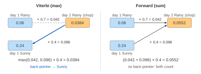
| Viterbi | Forward | |
|---|---|---|
| combines candidates with | max | sum |
| cell means | best path ending here | all paths ending here |
| keeps back-pointers | yes | no |
| answer | most likely hidden sequence | P(observations) |
| cost | O(T·N²) | O(T·N²) |
Log-probabilities and underflow
Every day multiplies by numbers below 1, so the cells keep shrinking: about four times a day for these sequences. A 64-bit float cannot go below about 4.9·10−324: on 800 days of observations every cell becomes exactly 0, all cells tie and the back-pointers mean nothing. Real decoders store log δ instead: products become sums, and since log is increasing the max picks the same winner. Here the cells show log10; code usually uses the natural log, which gives the same path. (Demo: log-probabilities and underflow) The forward algorithm cannot simply take logs of a sum; it uses the log-sum-exp trick or rescales each column.
Greedy is not enough
A greedy decoder picks the best state for day 1, then each day the best next state from the one it already chose, and never goes back. On walk, shop, clean it picks Sunny, then Sunny (0.6·0.3 = 0.18 beats 0.4·0.4 = 0.16), then Rainy: P = 0.00864, worse than Viterbi's 0.01344. Being Rainy on day 2 costs a little but makes "clean" on day 3 much cheaper. Viterbi keeps the best path into every state of every day, so a choice that pays off later is never thrown away. (Demo: greedy vs Viterbi)
Where it is used
- Part-of-speech tagging: hidden tags (noun, verb, …), observed words.
- Speech recognition: hidden phonemes, observed audio frames (classic HMM recognizers).
- Gene finding: hidden coding / non-coding regions, observed DNA bases.
- Error-correcting codes: Viterbi first decoded convolutional codes in modems, mobile phones and space probes.
See also Longest Common Subsequence and Dynamic Programming: Making Change for the same fill-a-table idea, Bayesian Networks for probabilistic inference in general, Naive Bayes for emission-style likelihoods and log-probabilities, and RNN and LSTM for the neural-network way of modelling sequences.
The hidden states follow a Markov chain; see how such a chain evolves and settles in Markov Chains and Random Walks.
See also Decoding Strategies: beam search keeps only the k best paths instead of filling the whole trellis.
What the page leaves out
Learning π, a and b from data (Baum–Welch, the forward–backward algorithm); the backward pass and per-day posterior probabilities; more than two states and continuous observations (Gaussian emissions); beam search and other pruning that real speech decoders need; higher-order HMMs and conditional random fields; and the log-sum-exp arithmetic for the forward algorithm.