The idea: tomorrow depends only on today
A Markov chain is a set of states and, for every state, the probabilities of where to go next. Here the states are the weather: Sunny, Cloudy and Rainy. One hop is one day. If today is Sunny, tomorrow is Sunny with probability 0.6, Cloudy with 0.3 and Rainy with 0.1. What happened before today does not matter. That is the Markov property.
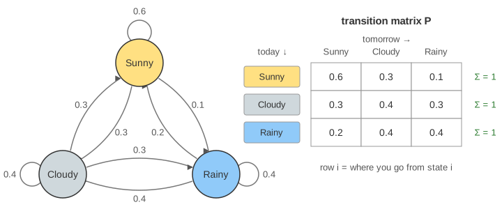
The probabilities form the transition matrix P. Row i is "today is i", column j is "tomorrow is j". Each row is a probability distribution, so it sums to 1.
A walker: one random path
Put a walker on Sunny and let it hop. Each day draw a random number u in [0, 1) and cut today's row into slices: for Sunny, u < 0.6 means Sunny, 0.6 ≤ u < 0.9 means Cloudy, and u ≥ 0.9 means Rainy. The page uses a seeded generator, so the path is random but repeatable. The visits panel counts how many days the walker spent in each state. (Demo 1: walker hops, visit counts: after 1 000 hops the shares are 0.412, 0.354 and 0.235.)
The shares settle down as the walk gets longer. They do not depend on where the walker started, and they are not 1/3 each: Sunny is "stickier" (0.6 to stay), so the walk spends more days there.
All paths at once: π ← π · P
Instead of one walker, track the distribution π: the chance of each state on day t. If π = (a, b, c) today, the chance of Sunny tomorrow adds up every way to get there:
That is the row vector π times column 1 of P. Doing it for every column is one vector–matrix product: πt+1 = πt · P, so πt = π0 · Pt (see Matrix Multiplication). Starting from Sunny, π0 = (1, 0, 0), π1 = (0.6, 0.3, 0.1) is just row Sunny, and π2 = (0.47, 0.34, 0.19). (Demo 2: distribution evolving writes each product out.)
Two starts, one limit
Start A begins on a Sunny day, start B on a Rainy day. Their bars look nothing alike at first, but each day the gap shrinks, and after about 10 days they agree to 4 decimals. (Demo 3: two starts converge: the largest gap after 10 days is 0.0001.)
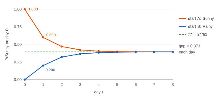
The chain forgets its start because every state can reach every other (irreducible) and it does not cycle with a fixed period (aperiodic). Under those two conditions every start converges to the same distribution.
The stationary distribution: πP = π
The limit is a distribution that one more day does not change. Call it π*. It solves π* · P = π* with the entries summing to 1:
| Equation | Meaning |
|---|---|
| S = 0.6S + 0.3C + 0.2R | flow into Sunny = share of Sunny |
| R = 0.1S + 0.3C + 0.4R | flow into Rainy = share of Rainy |
| S + C + R = 1 | it is a distribution |
The answer is π* = (24/61, 22/61, 15/61) ≈ (0.393, 0.361, 0.246). The walker's long-run visit shares match it too (ergodic theorem): the average over time equals the average over the distribution. (Demo 4: stationary distribution draws π* as green lines on both the bars and the visit shares.)
In linear-algebra terms, π* is a left eigenvector of P with eigenvalue λ = 1 (see Eigenvectors). Every stochastic matrix has λ = 1, because its rows sum to 1. The other eigenvalues of this P are 0.2 ± √0.03 = 0.373 and 0.027. The gap to π* shrinks by the largest of them, 0.373, each day, which is why about 10 days are enough.
A random walk on a line: distance grows like √n
A walker on the integers steps +1 or −1 with probability ½ each. This is a Markov chain with infinitely many states. On average the steps cancel, so the expected position stays 0, but the walker still wanders off. The squared position grows by exactly 1 per step on average, so after n steps the root-mean-square distance is √n.
| Steps n | RMS distance of 1 000 walkers | √n |
|---|---|---|
| 16 | 3.93 | 4 |
| 64 | 7.76 | 8 |
| 144 | 11.86 | 12 |
Four times the steps only doubles the distance. The histogram of where the walkers end is a bell curve of width √n, the same √n as in the Central Limit Theorem. (Demo 5: 1D random walk.)
Absorbing states: gambler's ruin
A gambler with $3 bets $1 on fair coin flips and stops at $0 (broke) or $10 (goal). The cash is a random walk, but $0 and $10 are absorbing states: their row of P is all 0 except a 1 on the diagonal, so once there, the walk stays forever. This chain is not irreducible, and its long-run behaviour depends on the start.
A fair game keeps the expected cash at $3, so 3 = P(goal) · 10 and P(ruin) = 1 − k/N = 1 − 3/10 = 0.7. The expected length is k(N − k) = 3 · 7 = 21 bets. (Demo 6: gambler's ruin: the first game ends at $0 after 7 bets; over 1 001 games 687 end broke, 0.686, with 21.7 bets on average.)
Where Markov chains show up
- Hidden Markov models: the states are hidden and you only see noisy observations; Viterbi finds the most likely state path.
- Markov decision processes: add actions and rewards and choose the best action in each state; see Value Iteration and Q-Learning.
- PageRank: a random surfer clicks links; a page's rank is its share in the stationary distribution.
- Markov chain Monte Carlo: build a chain whose stationary distribution is the one you want to sample, like the Metropolis rule in Simulated Annealing (compare plain Monte Carlo).
- Text models: the next word drawn from the current word is a Markov chain over words.
See also the Monty Hall problem for conditional probability on a tree of two random steps.
What the page leaves out
Periodic and reducible chains in general, mixing times and the spectral gap, continuous-time chains, hitting and return times, recurrence and transience (a 1D or 2D walk always comes back, a 3D walk may not), biased gambler's ruin (P(ruin) with p ≠ ½), and how to compute π* for large chains by power iteration.