The idea: three answers to "what is typical?"
A list of numbers can be summed up by one "typical" value in three common ways. The mean is the balance point: add the values and divide by how many there are. The median is the middle value once the list is sorted: half the values are below it and half above. The mode is the value that appears most often. The page computes all three on the same data, drawn as a dot plot (one dot per value, equal values stacked). One Step does one unit of work in each lane, and a scoreboard under the lanes shows what each answer is good at.
Mean: sum ÷ n
The mean lane reads the values one at a time and keeps a running sum; its blue marker on the axis shows the mean so far. After the last value, one more step divides: mean = (x₁ + x₂ + … + xₙ) / n. If the dots were weights on a ruler, the mean is where the ruler balances: the distances to the left and right add up to the same total. So a value far out counts in proportion to how far out it is.
The mean is the only one of the three that keeps the total: n × mean = sum. The scoreboard's "n × value" column shows a ✓ only for the mean. That is why budgets, averages per person and expected values use it.
Median: the middle value
The median lane first sorts the values (the chips move into order). Then each step crosses off the lowest and the highest value left. When one value is left, it is the median; when two are left (an even count), the median is their average. The median only cares about order: the scoreboard's "below | above" column shows equal counts on each side for the median, and lopsided counts for the other two on skewed data.
Sorting costs more than one pass (about n log n comparisons; a selection algorithm can find the median in linear time, but it still has to look at every value more than once). The page draws the sort as one Step.
Mode: the most common value
The mode lane reads the same values as the mean lane and adds one to a tally bar per distinct value. After the last value it takes the tallest bar. Two bars of the same top height give two modes (bimodal data). If every bar is 1 high, no value repeats and there is no mode (Demo: every value different). The mode is the only one of the three that works for categories (colours, brands, shirt sizes), where there is nothing to add or sort.
Outliers: which one moves?
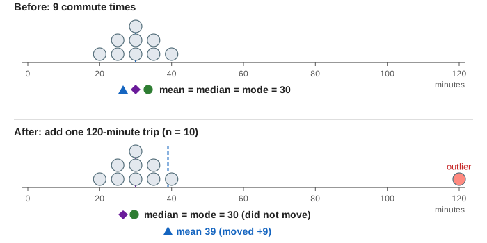
Nine commute times from 20 to 40 minutes are symmetric with one peak, and all three say 30 (Demo: symmetric commute times). Now add one trip of 120 minutes. The sum grows by 120, so the mean moves from 30 to 39. In the sorted order the new value only adds one chip at the right end, so the middle moves by at most half a place: the median stays 30. The 30 tally is still the tallest, so the mode stays 30 (Demo: add a 120-minute outlier). A statistic that one bad value cannot drag far is called robust; the median is the standard robust choice.
Skew and the order of the three
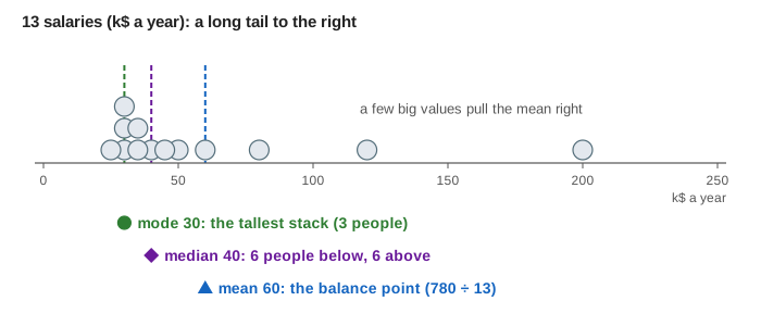
Salaries, house prices and waiting times have a long tail on the right: many modest values and a few large ones. On such right-skewed data the three spread out in the order mode < median < mean. In the salaries demo the mode is 30k, the median 40k and the mean 60k, and 9 of the 13 people earn less than the mean (Demo: right-skewed salaries). That is why news reports give the median household income: the mean describes nobody in particular. A left-skewed tail (a few very low values) reverses the order.
Two groups mixed together are worse. Café visits are either a quick take-away (5–15 minutes) or a sit-down (35–45 minutes). The mean and the median both come out at 25 minutes, and no visit lasted anywhere near 25: the "equal to it" column is 0 for both. Only the mode reports the two peaks, 5 and 45 (Demo: bimodal café visits). When the data has two peaks, show the dot plot or histogram, not one number.
When to pick which
| Mean | Median | Mode | |
|---|---|---|---|
| What it balances | distances: the values' total | counts: half below, half above | nothing: the tallest stack |
| One outlier | moves a lot ✗ | barely moves ✓ | does not move ✓ |
| Keeps the total (n × value = sum) | yes ✓ | no | no |
| Two peaks | lands in the gap ✗ | lands in the gap ✗ | finds both ✓ |
| All values different | fine | fine | no mode ✗ |
| Categories (colours, brands) | meaningless | only if the categories have an order | works ✓ |
| Work | one pass | a sort (or a selection algorithm) | one pass with a tally |
| Pick it when | the data is roughly symmetric, or you need totals and averages per item | the data is skewed or has outliers: incomes, prices, response times | you want the most common choice, or the data has several groups |
See also Normal Distribution, where mean, median and mode coincide at the centre of the bell, and Central Limit Theorem, where the mean of many values becomes normal even when the values are skewed.
What the page leaves out
The spread around the centre (range, quartiles, standard deviation), which a typical value alone cannot show. Also left out: weighted means, the trimmed mean (drop the top and bottom 10% first, a compromise between mean and median), geometric and harmonic means for rates, the modal class of grouped data in a histogram with bins, linear-time median selection (quickselect, median of medians), streaming estimates of the median for data too big to sort, and the mean, median and mode of continuous distributions.