Eigenvectors & Eigenvalues of a 2×2 Matrix

The idea: vectors that keep their direction

A 2×2 matrix A moves every vector of the plane: v goes to A·v. Draw a ring of unit vectors and apply A. The ring becomes an ellipse, and almost every arrow is turned off the line it was on. A few arrows are special: they stay on their own line and only get longer, shorter or flipped. Those are the eigenvectors.

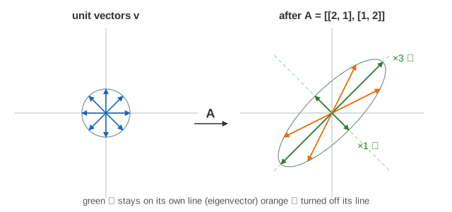
In symbols, v ≠ 0 is an eigenvector when A·v = λ·v for some number λ, its eigenvalue. The whole line through v is kept, so any multiple of v is an eigenvector too; the page shows unit-length ones. (Demo: symmetric [[2,1],[1,2]]: 4 of the 16 arrows stay green, on two lines, stretched ×3 and ×1.)

The characteristic equation

A·v = λ·v is the same as (A − λI)·v = 0. A non-zero v can only be sent to zero if the matrix A − λI squashes the plane flat, which means its determinant is 0 (see Determinant). For A = [[a, b], [c, d]]:

det(A − λI) = (a − λ)(d − λ) − b·c
            = λ² − (a + d)·λ + (a·d − b·c)
            = λ² − trace·λ + det = 0

This quadratic is the characteristic equation. Its discriminant Δ = trace² − 4·det decides what kind of eigenvalues A has:

Δ	Eigenvalues	Example on the page
Δ > 0	two different real λ, two eigen lines	[[2,1],[1,2]]: λ = 3, 1. [[3,1],[0,2]]: λ = 3, 2
Δ = 0	one repeated real λ	shear [[1,1],[0,1]]: λ = 1 twice
Δ < 0	a complex pair, no real eigenvector	rotation [[0,−1],[1,0]]: λ = ±i

Two handy checks: the eigenvalues add up to the trace and multiply to the determinant (3 + 1 = 4 and 3·1 = 3 for the symmetric example).

Finding the eigenvector

For each λ, solve (A − λI)·v = 0. Because det(A − λI) = 0, the two rows of A − λI are multiples of each other, so one row is enough: if a row is (p, q), then v = (−q, p) works. For λ = 3 in the symmetric example, A − 3I = [[−1, 1], [1, −1]] and v = (1, 1), or (0.707, 0.707) at unit length. For larger matrices this is Gaussian elimination on A − λI.

Symmetric, non-symmetric, rotation, shear

Matrix	What Multiply by A shows	Eigenvectors
Symmetric [[2,1],[1,2]]	ellipse along 45° and 135°	(0.707, 0.707) and (0.707, −0.707), perpendicular
Non-symmetric [[3,1],[0,2]]	a tilted ellipse	(1, 0) and (0.707, −0.707), at 45° to each other
Rotation [[0,−1],[1,0]]	the ring is turned 90°; every arrow is orange	none (λ = ±i)
Shear [[1,1],[0,1]]	the ring leans sideways	only (1, 0): one line for a double λ

A symmetric matrix always has real eigenvalues and perpendicular eigenvectors (the spectral theorem), which is why covariance matrices in statistics are so well behaved. A triangular matrix has its eigenvalues on the diagonal. A shear is defective: λ = 1 appears twice but A − I has rank 1, so there is only one eigen line. (Demos: non-symmetric, rotation, shear.)

Power iteration and the ratio |λ2/λ1|

Solving a quadratic only works for 2×2. For a large matrix, the classic way to get the biggest eigenvalue is power iteration: start from any vector, then repeat x ← A·x / ‖A·x‖. Write the start vector as c1·v1 + c2·v2. After k multiplications it is c1·λ1^k·v1 + c2·λ2^k·v2, so the v2 part shrinks relative to the v1 part by |λ2/λ1| every step. Normalising only keeps the numbers from blowing up.

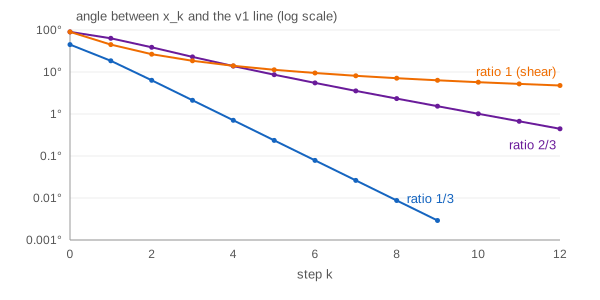
The table shows each x_k, the Rayleigh quotient xᵀAx (an estimate of λ1), the angle between x_k and the v1 line, and the ratio of successive errors. (Demo: power iteration, ratio 1/3: the ratio column settles at 0.333 and x₈ is within 0.01° of v1. Demo: ratio 2/3: the ratio settles near 0.667 and 12 steps still leave an error of about 0.4°.) If |λ1| = |λ2| there is no dominant direction: for the rotation, x just turns 90° per step forever, and for the shear it creeps towards (1, 0) like 1/k.

Where eigenvectors show up

• PageRank: the ranking is the dominant eigenvector of the link matrix, found by power iteration.
• PCA: the main directions of a data cloud are the eigenvectors of its covariance matrix.
• Optimisation: the eigenvalues of the Hessian set how fast gradient descent can go in each direction.
• Vibrations and Markov chains: natural modes and steady states are eigenvectors.

See also Vectors & Dot Product, Determinant, Gaussian Elimination and Changing Coordinates in 2D.

The eigenvectors of a covariance matrix are the principal axes in SVD and PCA, and the SVD gives every matrix perpendicular stretch directions. A Markov chain's stationary distribution is the eigenvector with λ = 1: see Markov Chains and Random Walks.

The axes of a tilted ellipse or hyperbola Ax² + Bxy + Cy² = 1 are the eigenvectors of [[A, B/2], [B/2, C]], and the eigenvalues set its width along them: see Conic Sections: What A, B, C, D, E, F Do.

What the page leaves out

Only 2×2 real matrices. Complex eigenvectors (a rotation does have them, in ℂ²), algebraic vs geometric multiplicity in general, diagonalisation A = PDP⁻¹, the QR algorithm that real libraries use for all eigenvalues at once, inverse and shifted power iteration for the other eigenvalues, and the singular value decomposition.

References

Gilbert Strang — Introduction to Linear Algebra, ch. 6: Eigenvalues and Eigenvectors

3Blue1Brown — Eigenvectors and eigenvalues (Essence of Linear Algebra)

Power iteration (Wikipedia)