The idea: make big weights cost something
A model with many weights can fit the noise in its training data. Regularization adds a penalty for large weights to the loss, so the fit has to trade a little training error for smaller weights. One knob, λ, sets how much the penalty counts. The two classic penalties are:
- L1 (lasso): minimise ½·MSE(w) + λ·(|w1| + |w2|).
- L2 (ridge): minimise ½·MSE(w) + ½·λ·(w1² + w2²).
The page fits the same data with both, at the same λ, one notch per Step. Each lane shows the loss contours in the (w1, w2) plane around the least-squares fit ŵ (★), the fit for the current λ (the big dot, with a trail behind it), and its two weights as bars, with the least-squares weights in grey behind them.
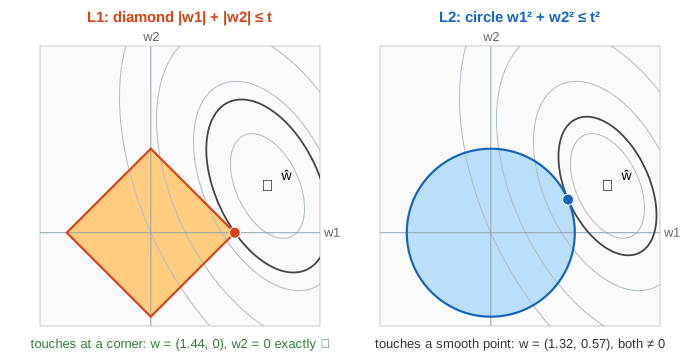
Why L1 gives exact zeros: the diamond's corners
Every penalized fit is also a constrained fit: the lowest loss among all w with |w1| + |w2| ≤ t (L1) or w1² + w2² ≤ t² (L2), for some size t that shrinks as λ grows. The L1 region is a diamond with corners on the axes; the L2 region is a circle. Grow the loss contours out from ★ until one touches the region: that point is the fit. Each lane draws the region in its colour and the touching contour in dark grey.
A pointed corner sticks out, so the contours very often hit the diamond at a corner, and a corner lies on an axis: one weight is exactly 0. The circle has no corners, so the touching point is almost never on an axis. (Demo: λ sweep: L1's w2 reaches 0 at λ = 1.00 and w1 at λ = 3.50; L2 at λ = 3.50 still has w = (0.75, 0.24).)
L1 (lasso): subtract, then clip at 0
With uncorrelated, standardized features, the lasso has a simple formula, soft thresholding: each weight's pull cⱼ (its correlation with y) loses λ, and if that crosses 0 the weight is 0.
wⱼ = sign(cⱼ) · max(|cⱼ| − λ, 0)          L1, uncorrelated features
wⱼ = ŵⱼ / (1 + λ)                         L2, uncorrelated features
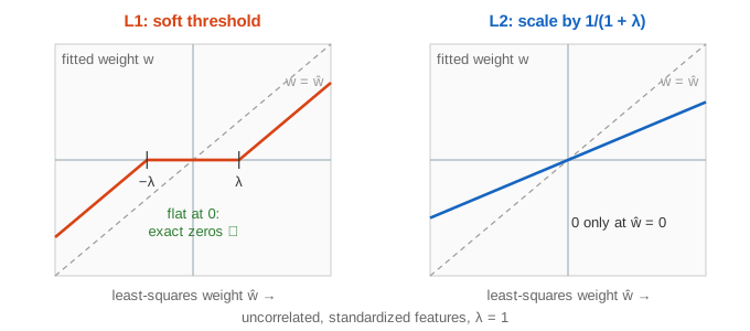
So the lasso does feature selection: once λ ≥ max |cⱼ|, every weight is 0 and the model predicts the mean of y. With correlated features there is no one-line formula; the page solves the 2-weight lasso exactly by trying every set of non-zero weights and keeping the one that meets the optimality (KKT) conditions. Real libraries use coordinate descent.
L2 (ridge): shrink everything a little
Ridge has a closed form, w = (XᵀX/n + λI)⁻¹ Xᵀy/n. Adding λ to the diagonal also makes the matrix well-conditioned, which is why ridge was invented: least squares with nearly collinear columns gives huge, unstable weights. Ridge weights shrink smoothly towards 0 but reach it only as λ → ∞.
Correlated features: pick one, or share
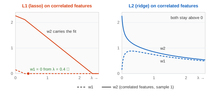
When x1 and x2 carry nearly the same information (here correlation 0.95), the contours become long, thin ellipses along w1 + w2 = const, and least squares can put almost all the weight on either feature depending on the noise. In Demo: correlated features least squares gives (0.15, 2.26) although the truth is (1.5, 1.5).
- L1 keeps one feature and drops the other (w1 = 0 from λ = 0.40). Which one survives depends on the sample: in Demo: a new sample, it keeps x1 and drops x2 instead.
- L2 pulls the two weights towards each other and shares the weight (about (0.87, 1.32) at λ = 0.2, and similar on the other sample). This grouping effect is more stable, and here it also predicts better: best test MSE 0.932 for L2 against 1.074 for L1.
Overfitting, and choosing λ
With only 8 training points and a useless second feature (Demo: 8 points + a useless feature), least squares fits the training points well (train MSE 0.803) but does badly on new data (test MSE 3.616): it is fitting noise. A moderate penalty helps both lanes: the best test MSE is 2.860 for L1 and 2.977 for L2, both at λ = 0.4, and from λ = 0.6 the lasso has removed the useless feature entirely. Push λ much further and both underfit (Demo: λ far too large): the L1 fit is all zeros, the L2 fit tiny, and both test errors are several times the no-penalty value. In practice λ is picked by cross-validation: try a grid of values and keep the one with the lowest error on held-out data. The page cheats a little by watching a test set directly.
When to pick which
| L1 (lasso) | L2 (ridge) | |
|---|---|---|
| Penalty | λ·Σ|wⱼ| | ½λ·Σwⱼ² |
| Constraint region | diamond (corners on the axes) | circle (ball) |
| Exact zeros | yes: feature selection, sparse model | no: every weight stays |
| Correlated features | keeps one, unstable choice | shares the weight, stable |
| Solution | no closed form; coordinate descent, LARS | closed form (XᵀX + λI)⁻¹Xᵀy; smooth, easy for gradient descent |
| Pick it when | you expect few useful features, or need a small model | many small effects, or collinear features |
Elastic net adds both penalties, λ·(α·Σ|wⱼ| + ½(1 − α)·Σwⱼ²): it keeps the lasso's zeros but selects correlated features in groups. In neural networks, L2 on the weights is called weight decay, because each gradient descent step first multiplies the weights by 1 − ηλ.
See also Linear & Logistic Regression (the unpenalized fit and the MSE) and Least Squares as Projection (the normal equations that ridge modifies).
Dropout is another regularizer: see Dropout & Batch Normalization.
What the page leaves out
Only two weights, so the picture can be drawn; with many features the diamond becomes a cross-polytope with even more corners, and the lasso keeps at most n non-zero weights. The intercept is not penalized and the features are standardized first, as libraries recommend, because the penalty depends on each feature's scale. The page also leaves out cross-validation itself, the Bayesian view (L2 is a Gaussian prior on the weights, L1 a Laplace prior), elastic net, group lasso, L0 / best-subset selection, dropout and early stopping, and the exact λ scalings of each library (scikit-learn's Ridge uses alpha = n·λ for the same fit).