Laplace Transform Visualization | F(s) as an Area, Poles, Solving ODEs

The idea: weigh f(t), then take the area

The Laplace transform turns a function of time f(t) into a function of a new variable s:

F(s) = ∫₀^∞ f(t)·e^(−st) dt

Read it as a recipe. Pick a number s. Multiply f(t) by the weight e^−st, a curve that starts at 1 and dies away, faster for bigger s. Then take the area under the product from t = 0 to ∞. That area is one number, F(s). Do it for every s and you get the whole function F.

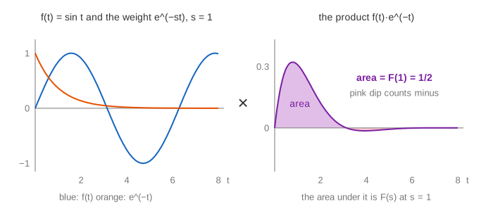
Left: f(t) = sin t in blue and the weight e to the minus t in orange. Right: their product, a hump that dies away, with the area under it shaded; the area is F(1) = 0.5 — f(t) times the weight e^−st gives a curve that dies out; the area under it is F(s). Here f = sin t and s = 1: F(1) = 1/2.

On the page the area is filled with strips of width 0.5 from t = 0 to 10, in four groups, with the exact running total beside them. The part after t = 10 is the tail; it is added from the formula. For f = 1 and s = 1 the area is exactly 1. (Demo 1)

Bigger s, smaller area

A bigger s makes the weight die faster, so less of f(t) counts and the area shrinks. Plot one dot per s and the dots trace F(s). (Demo 2: sweep s) The common pairs:

f(t)	F(s)	converges for	F(1)	F(2)
1	1/s	s > 0	1	0.5
t	1/s²	s > 0	1	0.25
e^−t	1/(s + 1)	s > −1	0.5	0.333
sin t	1/(s² + 1)	s > 0	0.5	0.2
e^t	1/(s − 1)	s > 1	∞	1
e^at	1/(s − a)	s > a
e^at·cos bt	(s − a)/((s − a)² + b²)	s > a

For sin t the product has a positive hump and smaller negative ones that partly cancel; the net area at s = 1 is 0.5. (Demo 3) For f = 1 the integral is easy by hand: ∫₀^∞ e^−st dt = [−e^−st/s]₀^∞ = 1/s.

Region of convergence and poles

The area only exists if the weight beats f. For f = e^t the product is e^(1−s)t. With s = 0.5 it grows like e^0.5t, with s = 1 it is the constant 1, and in both cases the area is infinite. Only for s > 1 does it die out, and then F(s) = 1/(s − 1). (Demo 4)

The set of s where the integral is finite, here s > 1, is the region of convergence. At its edge F(s) blows up: s = 1 is a pole of F. Every function the page uses grows at most like e^at, so each has a transform for s large enough.

Derivatives become multiplication by s

This is why engineers use the transform. Integrate by parts:

L{y′} = ∫₀^∞ y′(t)·e^(−st) dt = [y·e^(−st)]₀^∞ + s·∫₀^∞ y·e^(−st) dt = sY(s) − y(0)
L{y″} = s·L{y′} − y′(0) = s²Y(s) − s·y(0) − y′(0)

A derivative in t is a multiplication by s, minus the starting value. The transform is also linear: L{a·f + b·g} = a·F + b·G. So a linear differential equation with constant coefficients becomes an algebra equation for Y(s), and the start values y(0), y′(0) are already in it.

Solving an ODE in four moves

Transform every term with the rules above.
Solve for Y(s): collect the Y terms and divide. It is a fraction of two polynomials.
Split it into partial fractions, simple terms like 2/(s + 1). The cover-up rule finds each top number: cover the factor (s + 1) and put s = −1 in what is left.
Transform back, term by term, by reading the table from right to left: 1/(s − a) comes from e^at.

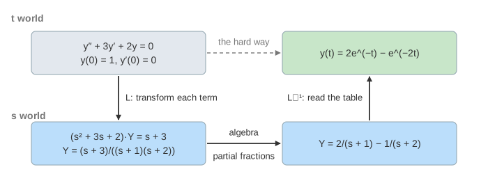
Two rows. Top row, the t world: the ODE y double prime plus 3 y prime plus 2 y equals 0 with start values, and its solution 2 e to the minus t minus e to the minus 2t. Bottom row, the s world: Y(s) = (s + 3)/((s + 1)(s + 2)) and 2/(s + 1) − 1/(s + 2). Arrows: the Laplace transform goes down, algebra goes across, the inverse transform goes up — Hard calculus in t becomes algebra in s: transform down, solve across, transform back up.

For y″ + 3y′ + 2y = 0 with y(0) = 1, y′(0) = 0: (s²Y − s) + 3(sY − 1) + 2Y = 0, so Y = (s + 3)/((s + 1)(s + 2)) = 2/(s + 1) − 1/(s + 2), and y(t) = 2e^−t − e^−2t. (Demo 5) A constant input on the right becomes c/s: y′ + 2y = 4 with y(0) = 0 gives Y = 4/(s(s + 2)) and y = 2 − 2e^−2t, which rises and settles at 2. (Demo 8) The same equations solved step by step numerically are in Euler's Method.

The poles tell the story

The poles of Y(s), where its bottom is zero, each give one term of y(t). A real pole a gives e^at. A complex pair a ± bi gives e^at·cos bt or e^at·sin bt. So the place of a pole on the s-plane says how y behaves:

pole	term in y(t)	behaviour	on the page
real, negative: −1, −2	e^−t, e^−2t	dies away, no swing	Demo 5
complex, left half: −1 ± 2i	e^−t·cos 2t	swings and dies away	Demo 6
at 0	a constant	stays	Demo 8
on the imaginary axis: ± bi	cos bt	swings forever
right half: +1	e^t	grows without bound	Demo 7

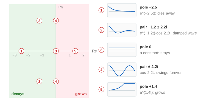
The s-plane with the left half shaded green and the right half red. Five poles are marked, each with a small sketch of its term in y(t): a real negative pole decays, a complex pair in the left half is a damped wave, a pole at 0 is a flat line, a pair on the imaginary axis is a steady wave, and a real positive pole grows — Left of the imaginary axis everything dies out; on it, it lasts; right of it, it grows. The imaginary part sets how fast it swings.

One pole on the right is enough to make the whole solution blow up: y″ − y = 0 has poles ±1, and y = cosh t = ½e^t + ½e^−t grows. (Demo 7) This is how control engineers test a system for stability: all poles in the left half. Demo 6 is a damped spring; the meaning of each number in e^−γt·cos ωt is in Damped Oscillation.

Laplace and Fourier

Put s = iω, a pure imaginary number, and the weight e^−iωt no longer dies out; it spins. The integral then measures how much of the frequency ω is in f: that is the Fourier transform (see Fourier Series and the FFT). The real part of s adds the decay that makes the integral converge even for functions that grow, like e^t. Complex numbers and e^iθ are explained in Complex Numbers; integrals to ∞ in Improper Integrals.

What the page leaves out

The page computes F(s) only for real s; F is really a function of complex s, and the general inverse is a contour integral (the Bromwich integral), not a table. Repeated poles (terms like 1/(s + 1)², which give t·e^−t), the convolution theorem (L{f * g} = F·G), transfer functions and Bode plots, the shift rules, the delta function and inputs that switch on later, the final-value theorem, and the two-sided transform are not shown.