Euler's Method: Follow the Slope Field

The idea: the equation tells you the slope everywhere

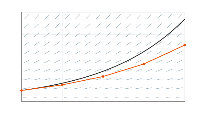
A differential equation such as y′ = f(t, y) does not give y directly. It says how fast y changes: at every point (t, y) the solution passing through it has slope f(t, y). Draw a short segment with that slope at many points and you get a slope field. A solution is a curve that follows the segments everywhere. Together with a start value y(0) (an initial value problem) the curve is fixed.

Euler's step

Euler's method walks the field with straight segments. From the point (t_n, y_n) it reads the slope there and follows it for a time h (the step size):

y_n+1 = y_n + h·f(t_n, y_n),   t_n+1 = t_n + h

This is the tangent line used as a prediction, the same idea as the derivative as a limit read backwards: f(t + h) ≈ f(t) + h·f′(t) for small h. For y′ = y, y(0) = 1 and h = 0.5 each step multiplies y by 1.5: 1, 1.5, 2.25, 3.375, 5.0625. The exact solution is y = e^t (see exponentials and logarithms). The curve bends upward, so a straight step always lands below it: Euler undershoots, and the gap grows. (Demo: slope field + Euler for y′ = y)

Error and order: halve h, halve the error

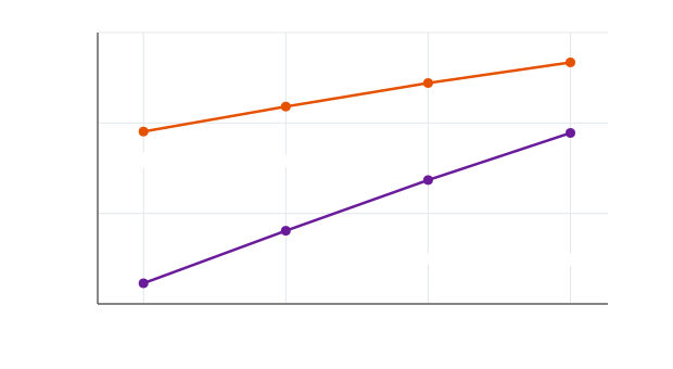
Smaller steps follow the curve more closely. Each step makes a local error of about h² (the curvature the straight line misses). Reaching a fixed time T takes T/h steps, so the global error at T is about (T/h)·h = T·h: proportional to h. Euler's method is first order: halving h halves the error, and also doubles the work. The canvas's error table for y′ = y at t = 1 (exact e ≈ 2.71828):

h	steps	Euler y(1) = (1 + h)1/h	error	error ratio	Heun error	Heun ratio
0.5	2	2.25	0.468		0.0777
0.25	4	2.4414	0.277	1.69	0.0234	3.31
0.125	8	2.5658	0.152	1.82	0.00644	3.64
0.0625	16	2.6379	0.0804	1.90	0.00169	3.81

The ratios approach 2 as h shrinks. (Euler's y(1) here is (1 + h)^1/h, the limit that defines e.) (Demo: halve h, the error at t = 1 halves)

Stability: too large a step blows up

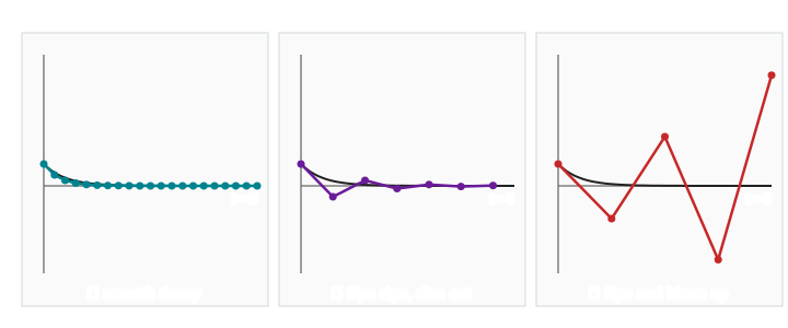
For the decay equation y′ = −2y (exact y = e^−2t) one Euler step gives y_n+1 = y_n − 2h·y_n = (1 − 2h)·y_n. The numbers shrink only when |1 − 2h| < 1, that is h < 1:

h	factor 1 − 2h	y0, y1, y2, …	behaviour
0.25	0.5	1, 0.5, 0.25, 0.125, …	✓ smooth decay
0.75	−0.5	1, −0.5, 0.25, −0.125, …	✓ flips sign every step, but dies out
1.25	−1.5	1, −1.5, 2.25, −3.375, 5.06	✗ flips sign and grows: unstable

The true solution decays for every h; the blow-up is created by the method. Equations with fast decay (stiff equations) force explicit methods like Euler to take tiny steps. Implicit methods such as backward Euler, y_n+1 = y_n + h·f(t_n+1, y_n+1), are stable for any h here. (Demo: decay, stable vs unstable h)

Logistic growth

The logistic equation y′ = y(1 − y) models a population that grows like y′ = y while small but levels off at the carrying capacity y = 1, where the slope field is flat. From y(0) = 0.1 the exact solution is the S-curve y = 1/(1 + 9e^−t). Euler with h = 1 runs ahead of the curve (0.19, 0.34, 0.57, 0.81, 0.97, …) but still settles at 1; with h = 0.25 it stays close. (Demo: logistic growth)

A better step: Heun's method

Euler uses only the slope at the start of the step. Heun's method (improved Euler, a two-stage Runge–Kutta method) first takes a trial Euler step, reads the slope at its end, and then steps with the average:

k₁ = f(t_n, y_n),  k₂ = f(t_n + h, y_n + h·k₁),  y_n+1 = y_n + h·(k₁ + k₂)/2

It costs two slope evaluations per step, but its error is proportional to h²: the table's Heun ratios approach 4. For y′ = y with h = 0.5 it reaches y(2) ≈ 6.97 instead of Euler's 5.06 (exact 7.39). Averaging slopes is the trapezoid rule from Riemann sums; the classic fourth-order Runge–Kutta method (RK4) averages four slopes and has error ∝ h⁴. (Demo: Euler vs Heun)

See also Newton's method, which also replaces a curve by its tangent line, there to find a root; Taylor series, whose first-order polynomial is exactly Euler's step; and the fundamental theorem of calculus: for y′ = f(t) alone, Euler's method is a left Riemann sum.

A spring with friction, m y″ + c y′ + k y = 0, has the exact solution A·e^(−γt)·cos(ωt + φ); what each number does is on Damped Oscillation: What A, γ, ω, φ Do.

For linear equations with constant coefficients there is an exact route too: the Laplace transform turns y′ and y″ into multiplication by s and the equation into algebra. See The Laplace Transform.

The four RK4 slopes, the midpoint method and an orbit where Euler spirals outward while RK4 stays on the circle are on Runge–Kutta vs Euler.

Take the logistic growth equation in steps as large as a whole generation and you get the logistic map, which can oscillate and turn chaotic: see The Logistic Map: from a Fixed Point to Chaos.

What the page leaves out

Only one equation in one unknown is shown. Systems of equations (a pendulum, predator and prey, planetary orbits) step a whole vector at once with the same formula. Real solvers such as RK45 change h as they go, using two methods of different order to estimate the error of each step. Backward Euler and other implicit methods are only described, and rounding error, which grows when h gets extremely small, is ignored.

References

Euler method (Wikipedia)

Paul's Online Math Notes: Euler's Method

Heun's method (Wikipedia)

Stiff equation (Wikipedia)