The idea: a polynomial that copies the derivatives
Near one point, a smooth function can be replaced by a polynomial. The Taylor polynomial of degree n at a point a is the polynomial whose value and first n derivatives at a are the same as the function's. When a = 0 it is also called a Maclaurin polynomial, and this page always uses a = 0:
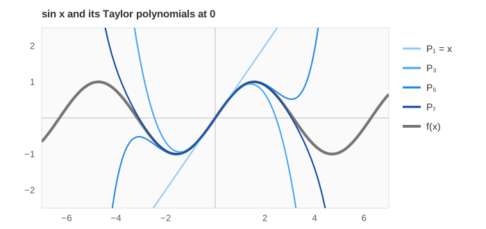
P(x) = f(0) + f′(0)·x + f″(0)/2!·x² + f‴(0)/3!·x³ + … + f⁽ⁿ⁾(0)/n!·xⁿThe infinite sum is the Taylor series. Each extra term fixes one more derivative, so the polynomial follows the curve a little further away from 0. On the canvas the grey curve is f, the blue curve is P, and the green bar shows where the two are within 0.01 of each other. Add Term adds one term at a time; a demo keeps adding terms until P has the number chosen in terms n (10 to 100, 20 by default). It shows the first 10 terms one by one, then adds 10 at a time; the error table keeps the last 10 rows.
Why divide by k!
Differentiate xᵏ k times and you get k·(k−1)·…·1 = k!, a constant; every other power becomes 0 at x = 0. So the k-th derivative of P at 0 is ck·k!. For it to equal f⁽ᵏ⁾(0), the coefficient must be ck = f⁽ᵏ⁾(0)/k!. The bottom panel of the canvas does exactly this for each new term: take the derivative, put x = 0, divide by k!.
The eight series on the page
| f(x) | derivatives at 0 | series | converges for |
|---|---|---|---|
| sin x | 0, 1, 0, −1, 0, 1, … | x − x³/3! + x⁵/5! − … | every x |
| cos x | 1, 0, −1, 0, 1, … | 1 − x²/2! + x⁴/4! − … | every x |
| eˣ | 1, 1, 1, 1, … | 1 + x + x²/2! + x³/3! + … | every x |
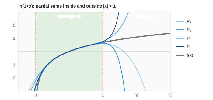
| ln(1+x) | 0, 1, −1, 2, −6, 24, … | x − x²/2 + x³/3 − … | −1 < x ≤ 1 |
| 1/(1−x) | 1, 1, 2, 6, 24, … (k!) | 1 + x + x² + x³ + … | −1 < x < 1 |
| arctan x | 0, 1, 0, −2, 0, 24, … | x − x³/3 + x⁵/5 − … | −1 ≤ x ≤ 1 |
| 1/(1+x²) | 1, 0, −2, 0, 24, … | 1 − x² + x⁴ − … | −1 < x < 1 |
| √(1+x) | 1, ½, −¼, ⅜, −15/16, … | 1 + x/2 − x²/8 + x³/16 − … | −1 ≤ x ≤ 1 |
The derivatives of sin and cos go round a cycle of four, so every other one is 0 at x = 0. Those terms are simply missing: sin x has only odd powers (it is an odd function) and cos x only even powers. The page skips the zero terms and counts only the ones that change P. (Demo 1: sin x, Demo 3: cos x)
How big is the error
The error after the degree-n term is the remainder R(x) = f(x) − P(x). Taylor's theorem in the Lagrange form says that, for some c between 0 and x,
R(x) = f⁽ⁿ⁺¹⁾(c) / (n+1)! · xⁿ⁺¹For sin, cos and eˣ the derivatives stay bounded on any interval, and (n+1)! grows faster than xⁿ⁺¹, so the error goes to 0 at every x. Far from 0 it takes more terms: at x₀ = 2, sin x needs degree 9 for an error of 5.0e−5, and eˣ needs 8 terms to get within 0.01 of e² = 7.389. The table on the canvas lists the error after each term. (Demo 2: eˣ)
The radius of convergence
Not every series works everywhere. ln(1+x) is not defined at x = −1, and that point limits its series in both directions: the series converges only for |x| < 1 (and at x = 1, slowly). This distance is the radius of convergence. Outside it the terms xᵏ/k grow, and each new term pushes P further away: at x₀ = 1.5 the error goes 0.58, 0.54, 0.58, 0.68, 0.84, 1.06, 1.38, 1.82. Inside, at x₀ = 0.5, it shrinks to 3.0e−5 after 10 terms. (Demo 4: ln(1+x))
The other three series with a finite radius show three different reasons for it:
- 1/(1−x), the geometric series, has every coefficient 1. It blows up at x = 1, so the radius is 1; at x₀ = 1.5 the partial sums 1, 2.5, 4.75, 8.125, … run off while f(1.5) = −2. (Demo 6: 1/(1−x))
- 1/(1+x²) is smooth on the whole real line, yet its series 1 − x² + x⁴ − … also stops at |x| = 1. In the complex plane 1 + x² = 0 at x = ±i, at distance 1 from 0, and the radius is the distance to the nearest such point. At x₀ = 1 the partial sums just flip between 1 and 0. (Demo 8: 1/(1+x²))
- √(1+x) is the binomial series with exponent ½. The square root ends at x = −1, so the radius is 1, but the coefficients shrink like k−3/2 and the series still converges at both ends. Its coefficients are not 1/k! any more: 1, ½, −⅛, 1/16, −5/128, 7/256, …. (Demo 9: √(1+x))
Computing e and π from partial sums
Put x = 1 into the series of eˣ and you get e = 1 + 1 + 1/2! + 1/3! + …. The partial sums are 1, 2, 2.5, 2.666667, 2.708333, 2.716667, 2.718056, 2.718254, 2.718279, 2.718282. After 10 terms the error is 3.0e−7: each new term divides it by roughly the next k. (Demo 5: e ≈ 2.71828)
arctan′ x = 1/(1+x²) = 1 − x² + x⁴ − …, so integrating term by term gives arctan x = x − x³/3 + x⁵/5 − …. At x = 1, where arctan 1 = π/4, this is the Leibniz series π/4 = 1 − 1/3 + 1/5 − …. It converges, but very slowly: 4 × the sum of 10 terms is 3.041840 and of 100 terms 3.131593, still 0.01 short of π. The error after n terms is about 1/(4n), not the factorial speed of e. (Demo 7: arctan x)
Where it is used
- Small-angle approximations: sin x ≈ x and cos x ≈ 1 − x²/2 for small x, used in physics (the pendulum) and in graphics.
- Maths libraries reduce x to a small range first, then evaluate a short polynomial: near 0 a few terms are enough.
- Newton's method replaces f by its degree-1 Taylor polynomial, the tangent line, and solves that instead. See Newton's Method.
- A Fourier series is the other big way to write a function as a sum: sines that fit the whole period instead of powers that fit one point. See Fourier Series and the FFT.
The derivatives themselves are limits of difference quotients: see The Derivative as a Limit.
Euler's step is the first-order Taylor polynomial; see Euler's method. e can also be reached as the limit of compound interest (1 + 1/n)ⁿ: see Exponentials and Logarithms.
The integral test ties ∑ 1/nᵖ to ∫₁^∞ 1/xᵖ, which converges only for p > 1: see Improper Integrals.
The first two Taylor terms are the tangent line, the linear approximation in Local Linearity: Zoom In.
The simplest power series is the geometric series 1/(1 − x) = 1 + x + x² + …, which works exactly for |x| < 1; see geometric series.
A Fourier series approximates a periodic function over a whole period with sines and cosines instead of powers of x: see Fourier Series, Harmonic by Harmonic.
What the page leaves out
Series around a point a ≠ 0, in powers of (x − a). Complex numbers in general: the page only uses them to explain why 1/(1+x²) has radius 1, and does not plot anything off the real line. Functions like e−1/x² whose Taylor series at 0 is all zeros but which are not zero. And the better polynomials real libraries use: minimax and Chebyshev fits that spread the error over a whole interval.